Tutorial 2. Advanced capabilities of the MeasurementControl

See also

The complete source code of this tutorial can be found in

Tutorial 2. Advanced capabilities of the MeasurementControl.ipynb

Tutorial 2. Advanced capabilities of the MeasurementControl.py

Following this Tutorial requires familiarity with the core concepts of Quantify, we highly recommended to consult the (short) User guide before proceeding (see Quantify documentation). If you have some difficulties following the tutorial it might be worth reviewing the User guide!

We highly recommended to begin with Tutorial 1. Controlling a basic experiment using MeasurementControl before proceeding.

In this tutorial, we will explore the more advanced features of Quantify. By the end of this tutorial, we will have covered:

• Using hardware to drive experiments

• Software averaging

• Interrupting an experiment

import os
import signal
import sys
import time

import numpy as np
from lmfit import Model
from qcodes import ManualParameter

import quantify_core.visualization.pyqt_plotmon as pqm
from quantify_core.data.handling import set_datadir
from quantify_core.measurement.control import MeasurementControl
from quantify_core.utilities.examples_support import default_datadir
from quantify_core.visualization.instrument_monitor import InstrumentMonitor

rng = np.random.default_rng(seed=222222)  # random number generator

%matplotlib inline

Before instantiating any instruments or starting a measurement we change the directory in which the experiments are saved using the set_datadir() [get_datadir()] functions.

Tip: What data directory should I use?

We highly recommended to settle for a single common data directory for all notebooks/experiments within your measurement setup/PC (e.g. ~/quantify-data (unix) or D:\\quantify-data (Windows). The utilities to find/search/extract data only work if all the experiment containers are located within the same directory.

set_datadir(default_datadir())  # change me!

Data will be saved in:
/home/slavoutich/quantify-data

meas_ctrl = MeasurementControl("meas_ctrl")
plotmon = pqm.PlotMonitor_pyqt("plotmon_meas_ctrl")
meas_ctrl.instr_plotmon(plotmon.name)
insmon = InstrumentMonitor("Instruments Monitor")

A 1D Batched loop: Resonator Spectroscopy

Defining a simple model

In this example, we want to find the resonance of some device. We expect to find it’s resonance somewhere in the low 6 GHz range, but manufacturing imperfections makes it impossible to know exactly without inspection.

We first create freq: a Settable with a Parameter to represent the frequency of the signal probing the resonator, followed by a custom Gettable to mock (i.e. emulate) the resonator. The Resonator will return a Lorentzian shape centered on the resonant frequency. Our Gettable will read the setpoints from freq, in this case a 1D array.

Note

The Resonator Gettable has a new attribute .batched set to True. This property informs the MeasurementControl that it will not be in charge of iterating over the setpoints, instead the Resonator manages its own data acquisition. Similarly, the freq Settable must have a .batched=True so that the MeasurementControl hands over the setpoints correctly.

# Note that in an actual experimental setup `freq` will be a QCoDeS parameter
# contained in a QCoDeS Instrument
freq = ManualParameter(name="frequency", unit="Hz", label="Frequency")
freq.batched = True  # Tells meas_ctrl that the setpoints are to be passed in batches


def lorenz(amplitude: float, fwhm: float, x: int, x_0: float):
    """Model of the frequency response."""
    return amplitude * ((fwhm / 2.0) ** 2) / ((x - x_0) ** 2 + (fwhm / 2.0) ** 2)


class Resonator:
    """
    Note that the Resonator is a valid Gettable not because of inheritance,
    but because it has the expected attributes and methods.
    """

    def __init__(self) -> None:
        self.name = "resonator"
        self.unit = "V"
        self.label = "Amplitude"
        self.batched = True
        self.delay = 0.0

        # hidden variables specifying the resonance
        self._test_resonance = 6.0001048e9  # in Hz
        self._test_width = 300  # FWHM in Hz

    def get(self) -> float:
        """Emulation of the frequency response."""
        time.sleep(self.delay)
        _lorenz = lambda x: lorenz(1, self._test_width, x, self._test_resonance)
        return 1 - np.array(list(map(_lorenz, freq())))

    def prepare(self) -> None:
        """Adding this print statement is not required but added for illustrative
        purposes."""
        print("\nPrepared Resonator...")

    def finish(self) -> None:
        """Adding this print statement is not required but added for illustrative
        purposes."""
        print("\nFinished Resonator...")


gettable_res = Resonator()

Running the experiment

Just like our Iterative 1D loop, our complete experiment is expressed in just four lines of code.

The main difference is defining the batched property of our Gettable to True. The MeasurementControl will detect these settings and run in the appropriate mode.

# At this point the `freq` parameter is empty
print(freq())

None

meas_ctrl.settables(freq)
meas_ctrl.setpoints(np.arange(6.0001e9, 6.00011e9, 5))
meas_ctrl.gettables(gettable_res)
dset = meas_ctrl.run()

Starting batched measurement...
Iterative settable(s) [outer loop(s)]:
	 --- (None) --- 
Batched settable(s):
	 frequency 
Batch size limit: 2000


Prepared Resonator...

100% completed | elapsed time:      0s | time left:      0s  last batch size:   2000  

100% completed | elapsed time:      0s | time left:      0s  last batch size:   2000  
Finished Resonator...

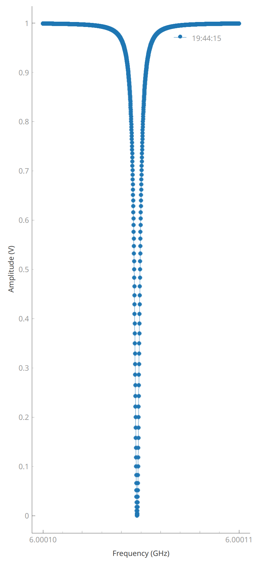
plotmon.main_QtPlot

As expected, we find a Lorentzian spike in the readout at the resonant frequency, finding the peak of which is trivial.

Memory-limited Settables/Gettables

Instruments (either physical or virtual) operating in batched mode have an upper limit on how many datapoints can be processed at once. When an experiment is comprised of more datapoints than the instrument can handle, the MeasurementControl takes care of fulfilling the measurement of all the requested setpoints by running and internal loop.

By default the MeasurementControl assumes no limitations and passes all setpoints to the batched settable. However, as a best practice, the instrument limitation must be reflected by the .batch_size attribute of the batched settables. This is illustrated below.

# Tells meas_ctrl that only 256 datapoints can be processed at once
freq.batch_size = 256

gettable_res.delay = 0.05  # short delay for plotting
meas_ctrl.settables(freq)
meas_ctrl.setpoints(np.arange(6.0001e9, 6.00011e9, 5))
meas_ctrl.gettables(gettable_res)
dset = meas_ctrl.run()

Starting batched measurement...
Iterative settable(s) [outer loop(s)]:
	 --- (None) --- 
Batched settable(s):
	 frequency 
Batch size limit: 256


Prepared Resonator...

 12% completed | elapsed time:      0s | time left:      0s  last batch size:    256  
 12% completed | elapsed time:      0s | time left:      0s  last batch size:    256  
Prepared Resonator...

Prepared Resonator...

Prepared Resonator...

Prepared Resonator...

Prepared Resonator...

Prepared Resonator...

Prepared Resonator...

100% completed | elapsed time:      0s | time left:      0s  last batch size:    208  

100% completed | elapsed time:      0s | time left:      0s  last batch size:    208  
Finished Resonator...

plotmon.main_QtPlot

Software Averaging: T1 Experiment

In many cases it is desirable to run an experiment many times and average the result, such as when filtering noise on instruments or measuring probability. For this purpose, the MeasurementControl.run() provides the soft_avg argument. If set to x, the experiment will run x times whilst performing a running average over each setpoint.

In this example, we want to find the relaxation time (aka T1) of a Qubit. As before, we define a Settable and Gettable, representing the varying timescales we will probe through and a mock Qubit emulated in software. The mock Qubit returns the expected decay sweep but with a small amount of noise (simulating the variable qubit characteristics). We set the qubit’s T1 to 60 ms - obviously in a real experiment we would be trying to determine this, but for this illustration purposes in this tutorial we set it to a known value to verify our fit later on.

Note that in this example meas_ctrl is still running in Batched mode.

def decay(t, tau):
    """T1 experiment decay model."""
    return np.exp(-t / tau)


time_par = ManualParameter(name="time", unit="s", label="Measurement Time")
# Tells meas_ctrl that the setpoints are to be passed in batches
time_par.batched = True


class MockQubit:
    """A mock qubit."""

    def __init__(self):
        self.name = "qubit"
        self.unit = "%"
        self.label = "High V"
        self.batched = True

        self.delay = 0.01  # sleep time in secs
        self.test_relaxation_time = 60e-6

    def get(self):
        """Adds a delay to be able to appreciate the data acquisition."""
        time.sleep(self.delay)
        rel_time = self.test_relaxation_time
        _func = lambda x: decay(x, rel_time) + rng.uniform(-0.1, 0.1)
        return np.array(list(map(_func, time_par())))

We will then sweep through 0 to 300 ms, getting our data from the mock Qubit. Let’s first observe what a single run looks like:

meas_ctrl.settables(time_par)
meas_ctrl.setpoints(np.linspace(0.0, 300.0e-6, 300))
meas_ctrl.gettables(MockQubit())
meas_ctrl.run("noisy")  # by default `.run` uses `soft_avg=1`
plotmon.main_QtPlot

Starting batched measurement...
Iterative settable(s) [outer loop(s)]:
	 --- (None) --- 
Batched settable(s):
	 time 
Batch size limit: 300


100% completed | elapsed time:      0s | time left:      0s  last batch size:    300  

100% completed | elapsed time:      0s | time left:      0s  last batch size:    300  

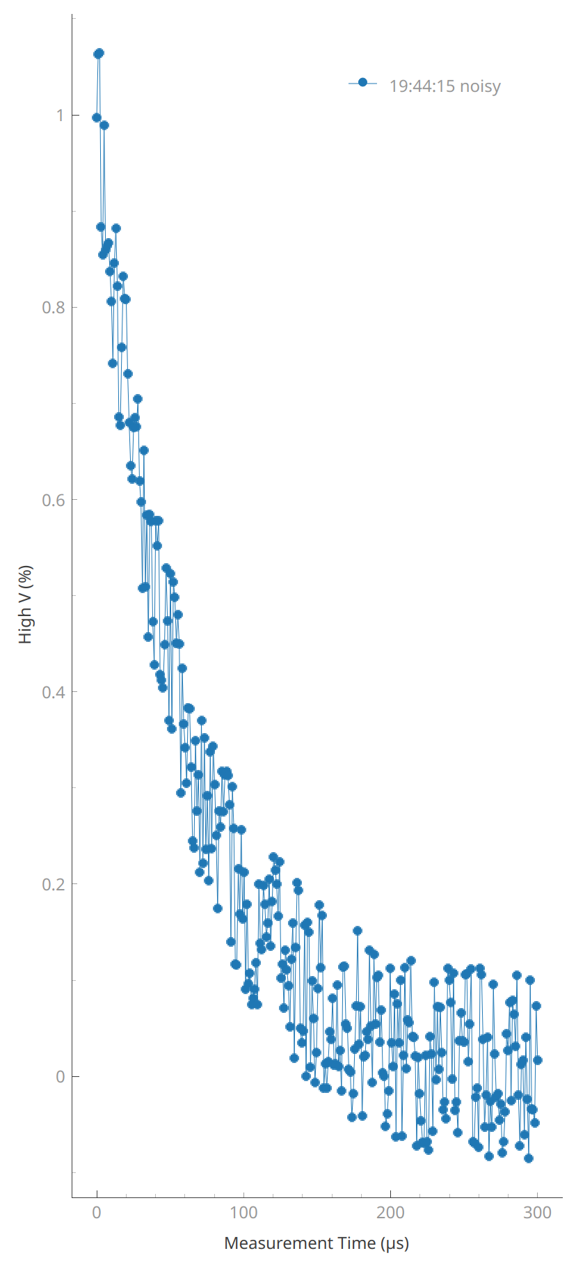
Alas, the noise in the signal has made this result unusable! Let’s set the soft_avg argument of the MeasurementControl.run() to 100, averaging the results and hopefully filtering out the noise.

dset = meas_ctrl.run("averaged", soft_avg=100)
plotmon.main_QtPlot

Starting batched measurement...
Iterative settable(s) [outer loop(s)]:
	 --- (None) --- 
Batched settable(s):
	 time 
Batch size limit: 300


  6% completed | elapsed time:      0s | time left:      2s  last batch size:    300  
  6% completed | elapsed time:      0s | time left:      2s  last batch size:    300  

 51% completed | elapsed time:      0s | time left:      0s  last batch size:    300  
 51% completed | elapsed time:      0s | time left:      0s  last batch size:    300  

 96% completed | elapsed time:      1s | time left:      0s  last batch size:    300  
 96% completed | elapsed time:      1s | time left:      0s  last batch size:    300  
100% completed | elapsed time:      1s | time left:      0s  last batch size:    300  

100% completed | elapsed time:      1s | time left:      0s  last batch size:    300  

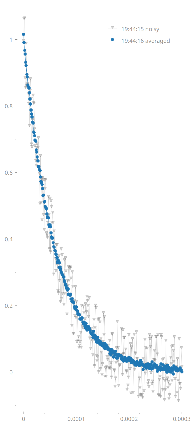
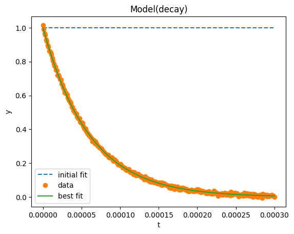
Success! We now have a smooth decay curve based on the characteristics of our qubit. All that remains is to run a fit against the expected values and we can solve for T1.

model = Model(decay, independent_vars=["t"])
fit_res = model.fit(dset["y0"].values, t=dset["x0"].values, tau=1)

fit_res.plot_fit(show_init=True)
fit_res.values

{'tau': 5.9945424534072186e-05}

Interrupting

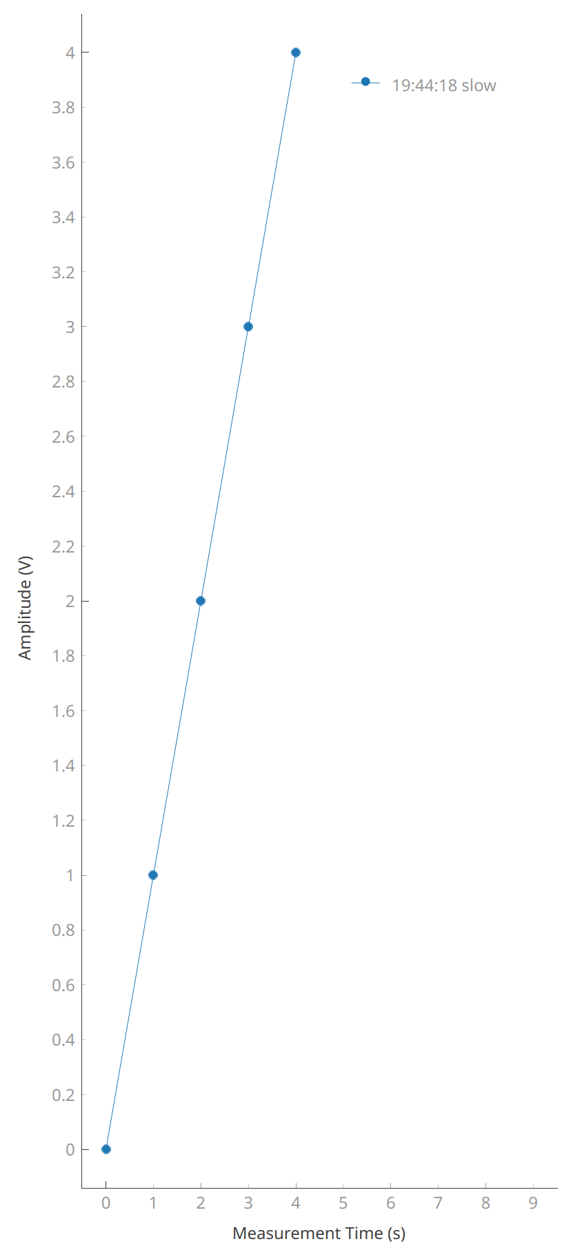
Sometimes experiments unfortunately do not go as planned and it is desirable to interrupt and restart them with new parameters. In the following example, we have a long running experiment where our Gettable is taking a long time to return data (maybe due to misconfiguration). Rather than waiting for this experiment to complete, instead we can interrupt any MeasurementControl loop using the standard interrupt signal. In a terminal environment this is usually achieved with a ctrl + c press on the keyboard or equivalent, whilst in a Jupyter environment interrupting the kernel (stop button) will cause the same result.

When the MeasurementControl is interrupted, it will wait to obtain the results of current iteration (or batch) and perform a final save of the data it has gathered, call the finish() method on Settables & Gettables (if it exists) and return the partially completed dataset.

Note

The exact means of triggering an interrupt will differ depending on your platform and environment; the important part is to cause a KeyboardInterrupt exception to be raised in the Python process.

Warning

In case the current iteration is taking too long to complete (e.g. instruments not responding), you may force the execution of any python code to stop by signaling the same interrupt 5 times (e.g. pressing 5 times ctrl + c). Mind that performing this too fast might result in the KeyboardInterrupt not being properly handled and corrupt the dataset!

class SlowGettable:
    """A mock slow gettables."""

    def __init__(self):
        self.name = "slow"
        self.label = "Amplitude"
        self.unit = "V"

    def get(self):
        """Get method."""
        time.sleep(1.0)
        if time_par() == 4:
            # This same exception rises when pressing `ctrl` + `c`
            # or the "Stop kernel" button is pressed in a Jupyter(Lab) notebook
            if sys.platform == "win32":
                # Emulating the kernel interrupt on windows might have side effects
                raise KeyboardInterrupt
            os.kill(os.getpid(), signal.SIGINT)
        return time_par()


time_par.batched = False
meas_ctrl.settables(time_par)
meas_ctrl.setpoints(np.arange(10))
meas_ctrl.gettables(SlowGettable())
# Try interrupting me!
dset = meas_ctrl.run("slow")

Starting iterative measurement...

 10% completed | elapsed time:      1s | time left:      9s  
 10% completed | elapsed time:      1s | time left:      9s  

 20% completed | elapsed time:      2s | time left:      8s  
 20% completed | elapsed time:      2s | time left:      8s  

 30% completed | elapsed time:      3s | time left:      7s  
 30% completed | elapsed time:      3s | time left:      7s  

 40% completed | elapsed time:      4s | time left:      6s  
 40% completed | elapsed time:      4s | time left:      6s  

[!!!] 1 interruption(s) signaled. Stopping after this iteration/batch.
[Send 4 more interruptions to forcestop (not safe!)].


 50% completed | elapsed time:      5s | time left:      5s  
 50% completed | elapsed time:      5s | time left:      5s  
Interrupt signaled, exiting gracefully...

---------------------------------------------------------------------------
KeyboardInterrupt                         Traceback (most recent call last)
Cell In [15], line 27
     25 meas_ctrl.gettables(SlowGettable())
     26 # Try interrupting me!
---> 27 dset = meas_ctrl.run("slow")

File ~/.local/opt/conda/envs/doc_qc064/lib/python3.9/site-packages/quantify_core/measurement/control.py:330, in MeasurementControl.run(self, name, soft_avg, lazy_set, save_data)
    327 self._finish()
    328 self._reset_post()
--> 330 self._check_interrupt()  # Propagate interruption
    332 return self._dataset

File ~/.local/opt/conda/envs/doc_qc064/lib/python3.9/site-packages/quantify_core/measurement/control.py:603, in MeasurementControl._check_interrupt(self)
    595 """
    596 Verifies if the user has signaled the interruption of the experiment.
    597 
    598 Intended to be used after each iteration or after each batch of data.
    599 """
    600 if self._thread_data.events_num >= 1:
    601     # It is safe to raise the KeyboardInterrupt here because we are guaranteed
    602     # To be running MC code. The exception can be handled in a try-except
--> 603     raise KeyboardInterrupt("Measurement interrupted")

KeyboardInterrupt: Measurement interrupted

plotmon.main_QtPlot